Quick Start Guide

Framework

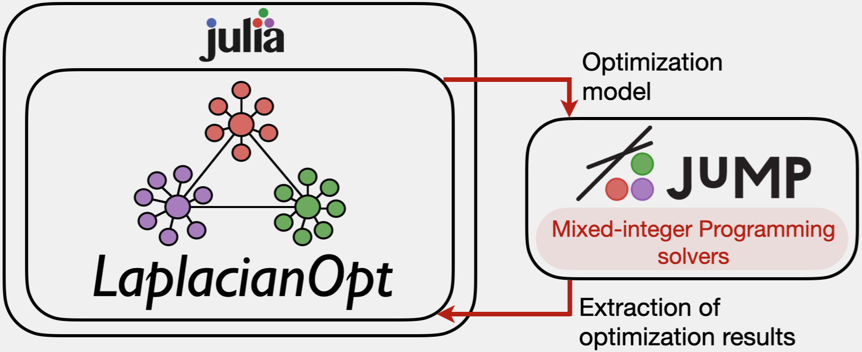
Building on the recent success of Julia, JuMP and mixed-integer programming (MIP) solvers, LaplacianOpt, is an open-source toolkit for the problem of maximum algebraic connectivity augmentation on graphs. As illustrated in the figure below, LaplacianOpt is written in Julia, a relatively new and fast dynamic programming language used for technical computing with support for extensible type system and meta-programming. At a high level, this package provides an abstraction layer to achieve two primary goals:

To capture user-specified inputs, such as the number of vertices of the graph, adjacency matrices of existing and augmentation graphs, and an augmentation budget, and to build a JuMP model of an MIP formulation with convex relaxations, and
To extract, analyze and post-process the solution from the JuMP model and to provide optimal connected graphs with maximum algebraic connectivity.

Getting started

After the installation of LaplacianOpt and a MIP solver, Gurobi.jl (use GLPK for an open-source MIP solver), from the Julia package manager, provide user inputs based on your available graph data. LaplacianOpt supports input data either in the JSON format, or by directly providing a data dictionary. Here, is an example on providing a data dictionary as an input. However, check this example script for providing data inputs using JSON files. A sample optimization model to maximize the algebraic connectivity of the weighted graph's Laplacian via edge augmentation can be executed with a few lines of code as follows:

import LaplacianOpt as LOpt
using JuMP
using Gurobi

function data()
    data_dict = Dict{String, Any}()
    data_dict["num_nodes"] = 4

    # Base graph with 3 existing edges (fixed). Note this graph can also be empty. 
    data_dict["adjacency_base_graph"] = [0 2 0 0; 2 0 3 0; 0 3 0 4; 0 0 4 0]

    # Augmentation graph with 3 candidate edges
    data_dict["adjacency_augment_graph"] = [0 0 4 8; 0 0 0 7; 4 0 0 0; 8 7 0 0]

    # Augmentation budget on candidate edges
    augment_budget = 2
    return data_dict, augment_budget
end

data_dict, augment_budget = data()

params = Dict{String, Any}(
    "data_dict"           => data_dict,
    "augment_budget"      => augment_budget
    )

lopt_optimizer = JuMP.optimizer_with_attributes(Gurobi.Optimizer, "presolve" => 1) 
results = LOpt.run_LOpt(params, lopt_optimizer)

Tip

Run times of LaplacianOpt's mathematical optimization models are significantly faster using Gurobi as the underlying mixed-integer programming (MIP) solver. Note that this solver's individual-usage license is available free for academic purposes.

Tip

Note that LaplacianOpt tries to find the global solution of a combinatiorial optimization problem, that is known to be NP-hard to compute in the size of num_nodes. To obtain quick feasible solutions via "k-opt-based" heristics, just set :solution_type to "heuristics" and adjust the num_swaps_bound_kopt parameter to appropriate values, where larger value implies a better-quality feasible solution at the cost of the heuristic run time.

Extracting results

The run commands (for example, run_LOpt) in LaplacianOpt return detailed results in the form of a dictionary. This dictionary can be used for further processing of the results. For example, for the given instance of a complete graph, the algorithm's runtime and the optimal objective value (maximum algebraic connectivity) can be accessed with,

results["solve_time"]
results["objective"]

The "solution" field contains detailed information about the solution produced by the optimization model. For example, one can obtain the edges of the optimal graph toplogy from the symmetric adjacency matrix with,

optimal_graph = LOpt.optimal_graph_edges(results["solution"]["z_var"])

Further, algebraic connectivity and the Fiedler vector of the optimal graph topology (though can be applied on any graph topology) can be obtained from the adjacency matrix with,

data = LOpt.get_data(params)
adjacency_matrix = data["adjacency_base_graph"] + data["adjacency_augment_graph"]
optimal_adjacency = results["solution"]["z_var"] .* adjacency_matrix 
graph_data = LOpt.GraphData(optimal_adjacency)
println("Algebraic connectivity: ", graph_data.ac)
println("Fiedler vector: ", graph_data.fiedler)

Visualizing results

LaplacianOpt also currently supports the visualization of optimal graphs layouts obtained from the results dictionary (from above. To do so, these are the two options:

TikzGraphs package for a simple and quick visualization of the graph layout without support to include edge weights, which can be executed with

data = LOpt.get_data(params)
LOpt.visualize_solution(results, data, visualizing_tool = "tikz")

Graphviz package for better visualization of weighted graphs. To this end, LaplacianOpt generates the raw .dot file, which can be further visualized using the Graphviz software either via the direct installation on the computer or using an online front-end visualization GUI (for example, see Edotor). Dot files can be generated in LaplacianOpt with

data = LOpt.get_data(params)
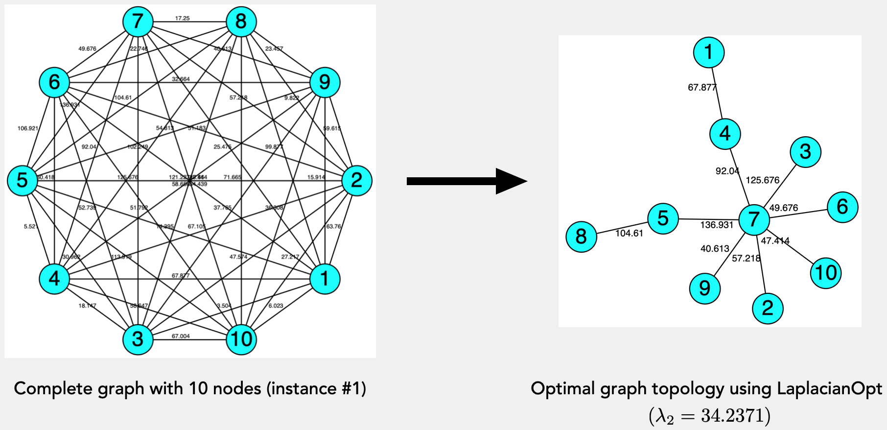
LOpt.visualize_solution(results, data, visualizing_tool = "graphviz")

For example, on a weighted complete graph with 10 nodes in instance #1, the optimal spanning tree with maximum algebraic connectivity, out of $10^8$ feasible solutions, obtained by LaplacianOpt (using Graphviz visualization) is shown below

Optimal solution